These notes were adapted for presentation from E. Stanley,
Introduction to Phase Transitions and Critical Phenomena,
D. Chandler, Introduction to Statistical Mechanics, and
Gould and Tabachnik, Introduction to Computer Simluations.
For an introduction into a thermodynamic version of RNG,
rather than real-space percolation example, please see
R.J. Creswick, H.A. Farach, C.P. Poole, Jr.,
Introduction to Renormalization Group Methods in Physics.
Note that while there is a correspondence between order parameters
in different physical systems there is no correspondence of the topology
of the individual phase diagrams. For example, for a fluid, P vs. T plot
corresponds to a M vs. T in a magnetic system, but the do not look alike.
In a magnetic systems H vs. T is a single line separating an "all up spin"
from an "all down spin" configuration, and TC is a the point
where the system obtains a non-zero M(T). Whereas, for a fluid there is a
critical point at the end of the vapor pressure curve where we can
continuously transform a gas to a liquid. These are not to be confused
with the curves which separate solid-gas (sublimation curve),
gas-liquid (vapor pressure curve), and the liquid-solid (fusion curve).
Therefore, such critical behavior can be manifest differently in any
particular cut of a (P,  , T) diagram or,
equivalently, a (H, M, T) diagram for a magnetic system.
Certainly, there are other types of global transitions, such
as in percolation, which result from a cluster spanning a system
and which occurs at some particular critical values of site
occupation probability, pC. So such critical behavior, and it
associated characteristics, are ubiquitous.
, T) diagram or,
equivalently, a (H, M, T) diagram for a magnetic system.
Certainly, there are other types of global transitions, such
as in percolation, which result from a cluster spanning a system
and which occurs at some particular critical values of site
occupation probability, pC. So such critical behavior, and it
associated characteristics, are ubiquitous.
A Correlation Length,  ,
is the distance over which a specific thermodynamic variable in
the system are correlated with one another and is relevant in a
system near a critical point, as evidenced
from the critical opalescence experiments.
In the 2-D Ising Model,
for example, you can see correlations of spins over larger and
larger distances as the TC is approached from above.
It becomes larger than the simulation box, L, rapidly near TC.
Above TC, such correlations of spins in the Ising model
show short-range order (correlations over short distances),
whereas below TC the system exhibits long-range order
(infinitely-ranged correlations).
,
is the distance over which a specific thermodynamic variable in
the system are correlated with one another and is relevant in a
system near a critical point, as evidenced
from the critical opalescence experiments.
In the 2-D Ising Model,
for example, you can see correlations of spins over larger and
larger distances as the TC is approached from above.
It becomes larger than the simulation box, L, rapidly near TC.
Above TC, such correlations of spins in the Ising model
show short-range order (correlations over short distances),
whereas below TC the system exhibits long-range order
(infinitely-ranged correlations).
Generally speaking, we observed three things near a critical point,
which are, in fact, interrelated. There is an
- increase in density fluctuations
As T  TC,
correlations become as large as the wavelength of light
TC,
correlations become as large as the wavelength of light
and the density inhomogeneities scatter light strongly
(critical opalescence).
- increase in compressibility
KT
 as T TC.
- increase in the range of the density-density correlations.
as T
TC.
Pair Correlations are clearly important, especially since
they are are directly related to thermodynamic quantities, such as KT.
With KT0 = <N>kT/V the ideal gas compressibility,
this is self-evident when we recall
KT/KT0 =
< (N - <N>)2 >/<N> and
< (N - <N>)2 > =
 dr
dr' G(r - r') =
V dr G(r)
As T TC,
KT
means that G(r - r') becomes very long
ranged, or G(r - r') 0 slowly as
|r - r'| >> 1. Hence, the connection between the density
fluctuations, compressibility and density-density correlations.
In addition, it is clear that the correlation length diverges
(
) at the critical point in order for
the density-density correlation to produce a divergent KT.
dr
dr' G(r - r') =
V dr G(r)
As T TC,
KT
means that G(r - r') becomes very long
ranged, or G(r - r') 0 slowly as
|r - r'| >> 1. Hence, the connection between the density
fluctuations, compressibility and density-density correlations.
In addition, it is clear that the correlation length diverges
(
) at the critical point in order for
the density-density correlation to produce a divergent KT.
The increased correlation length, and associated change in
thermodynamic quantities, lead to the concept of scaling in
a finite-sized simulation, in order to estimate the
proper critical points and
critical exponents.
Finite-size Scaling
Reduced Coordinates are often convenient to define
when discussing scaling of thermodynamic quantities.
For example, reduced temperature t = (T - TC)/TC,
which is a temperature relative to the critical point. You can
define reduced densities. Or, in percolation problems, reduced units would
be x = (p - pC)/pC.
Its use in what follows should be apparent.
Experimental Evidence for Scaling --
When measured coexistence curves of numerous fluids, e.g.,
are plotted as T/TC vs. /
C, a single curve is
found (see, e.g. E. Stanley, pg. 10). A fit to this curve reveals
that -
C ~
(-t) ,
and =0.33.
However, it is generally found that there is a range:
0.33 < < 0.37.
For example, in Helium, =0.354.
Measurements for other quantities, such as susceptibilities,
also lend themselves to this type of scaling analysis.
,
and =0.33.
However, it is generally found that there is a range:
0.33 < < 0.37.
For example, in Helium, =0.354.
Measurements for other quantities, such as susceptibilities,
also lend themselves to this type of scaling analysis.
Whether talking of magnetic systems, fluids, or percolation problems,
the order parameters (pair-correlations, correlation lengths, and so on)
exhibit this type of scaling behavior. Here we only discuss the named
quantities in the magnetic case, (i) Magnetization, M(T),
(ii) the isothermal susceptibility,  (T),
and (iii) the correlation length, (T),
and (iv) the zero-field specific heat, C(T).
For percolation, they would be the (i) spanning probability,
pinf, (ii) the mean cluster size, S(p), and
(iii) the correlation length, (p).
(T),
and (iii) the correlation length, (T),
and (iv) the zero-field specific heat, C(T).
For percolation, they would be the (i) spanning probability,
pinf, (ii) the mean cluster size, S(p), and
(iii) the correlation length, (p).
Scaling Properties and Critical Exponents
- Magnetization
M(T) ~ (-t)
0.33 < < 0.37.
(for T < TC)
- Magnetic Susceptibility
(T) ~
|t|- 1.3 < < 1.4.
- Correlation Length
(T) ~
|t|- depends on dimension of problem.
- Zero-field Specific Heat
C(T) ~ |t|- ~ 0.1.
The coefficients defining the power law behavior (i.e.,
, ,
, etc.) are referred
to as critical exponents
Scaling with Finite System Size
Consider a simulation system with linear dimension L.
Scaling revealed from behavior of Correlation Length
- If (T) < < L, power law behavior
is expected because the correlations are local and do not exceed L.
- If (T) ~ L, however,
cannot change appreciably and
M(T) ~ (-t)
is no longer applicable.
- For (T) ~ L ~
|t|-,
a quantitative change will occur in the system.
- This last relation obviously implies (for a given L) that
|T - TC(L)| ~ L-1/.
Scaling Relation of TC
Note that for a 2-dimensional system, like the square lattice,
=1. Thus, TC(L) should scale linearly
with L and the final TC should be (within error bars) close
to the exact 2-D square lattice in zero field, 2.269.
To determine TC(L), CV(L,T) vs. T is
calculated for various L = (4, 8, 16, 32, ...) and the maximum
CV(L,T) is used to indicate TC(L).
Recall CV(T) =
(<E2> - <E>2)/kT2, which
reveals the energy fluctuations of the system and the distribution of
configurations over energy, i.e. the more possible configurations,
the higher the specific heat.
Why not use
E vs. T plots to reveal the transition temperature, instead of
CV?
Determining the Critical Exponents
- From TC scaling relation
(when (T) ~ L
as L ),
M(T=TC(L)) ~
L-/ .
- A similar analysis may be made for susceptibility or specific heats.
- Or, for order paramters in other problems, such as percolation,
pinf(T=TC) ~
L-/ .
- Hence, the critical exponents can be determined through scaling analysis.
A Preliminary: Scaling Law for Homogeneous Functions
A function, f(r), is said to scale
if for all values of  ,
f( r) = g() f(r).
,
f( r) = g() f(r).
A function with this property is homogeneous, e.g.,
f(r)= Br2
f( r)= 2f(r),
and g()= 2.
For a homogeneous function, if we know f(r=r0)
and we know g(), then we know f(r) everywhere!
The scaling function is not arbitrary.
It must be g() =
P.
P is the degree of homogeneity.
See Stanley, pg 176 for "proof".
A generalized homogeneous function is given by
f(a x,
b y) =
f(x,y).
There is no P
on R.H.S. because you could always re-scale with
1/P and change a'=a/P
and b'=b/P, without loss of generality.
Notice this is NOT f( x,
y) =
P f(x,y),
as you might suspect, because functions can be
scaled differently in different directions.
Static Scaling Hypothesis for Thermodynamic Functions
The (ad hoc) static scaling hypothesis asserts that
G(t,H) is a generalized homogeneous function.
Hence, G(at t,
aH H) =
G(t,H).
If G(t,H) is a generalized homogeneous function,
then so are all other forms of Free Energy, as they
are just Legendre transforms of G.
Relations amongst critical exponents may be obtained
by application of thermodynamic relations, e.g.,
M(t,H) = -dG(t,H)/dH.
Taking this derivative, we find
(try it!):
aH
M(at t,
aH H) =
M(t,H).
For zero field,
M(t,0) = aH-1
M(at t, 0).
- Letting =
(- t-1)1/at yields the scaling
M(t,0) = (-t)(1-aH)/at M(-1,0)
- And, because we know M(t,0) ~
(-t), then
= (1-aH)/at .
- The same can be done for all observables which are derivatives of G(t,H).
- e.g. T ~
(-t)-' from below TC,
' = (2 - aH)/at.
- e.g. T ~
(t)- from above TC,
= (2 - aH)/at ,
and ' = .
From SCALING of the thermodynamic functions, the
critical exponents can be determined
in terms of ratios of only 2 quantities, aH and at.
Hence, by plotting the thermodynamic functions according to the derived
scaling relations, both aH and at can be determined.
You can perform the same type of analysis for other Thermodynamic
functions or quantities to derive the scaling equalities, which from
another analysis are given as inequalities (but you must remember
that the scaling hypothesis was, in fact, an ad hoc idea -- but
seems to be born out).
Renormalization Group
Because the correlation length diverges, and various fluctuation
grow (along with the associated pair correlations), as TC
is approached from above, it shows that long-range fluctuations
control the phase transition and the critical point. This also
suggests that the phase transition (or fluctuations) is associated with
the degree of connectivity of the system. Recall that there is no
connectivity in 1-D and, hence, no phase transition.
(You may have connectivity but in combination with frustration due, say,
to geometry of lattice and competing interactions which results in no
phase transition, as with the triangular lattice and AFM interactions.
But this is because there is no unique ground-state, not becuase of
non-connectivity.)
The results of scaling, as discussed above, is that the important
fluctuations and their range can be scaled up to the appropriate
lenght scale, and the local effects (which do not control the phase
transition) can be ignored. Such scaling ideas were developed by
Leo Kadanoff in the 60's in real space, which provided a very intuitive
insight. However, these ideas were still only approximate and not
complete. Nonetheless, the ideas of fixed points, Kadanoff
transformations, etc. extend directly into many areas of physics,
chemistry, and engineering (although perhaps not obvious at first glance).
Based on the work of Kadanoff, Ken G. Wilson in the early 70's proposed
a formal mathematical approach (based in reciprocal-space (or k-space))
solvable with large-scale computing, now known as the
Renormalization Group (RNG) Theory. For this work he was awarded
the Nobel Prize in Physics in 1982.
It has less intuitive nature than the so-called
Real-space Renormalization Group ideas of Kadanoff, but carries
the principals out exactly, in principle. Two good references for
an overview of these ideas are in Problems in Physics with Many
Scales of Length, Sci. Am. 241, 158 (1979) and
Rev. Mod. Phys. 55, 583 (1983) by K.G. Wilson.
A good introduction to the concepts of RNG can be found in
D. Chandler's Introduction to Modern Statistical Mechanics,
pg. 139. For statistical mechanics problems, the key issues is how
to re-scale the partition function such that it (i) retains the
same symmetry and ground-state given by the original partition function,
(ii) can re-scale the so-called coupling constant, i.e.
K = J/kT in the nearest-neighbor model, and (iii) the partition
function can be re-cast in terms of partially summed original
partition function such that it look the same as original,
with different spins and (perhaps) with different coupling constant.
If this re-scale is possible, then we can develop a
Recursion Relation to compute the partition function from a
system with another coupling (e.g., zero, non-interacting system).
An iterative solution of this Recursion Relation for the partition
function yields "roots" or fixed points of the solution space.
The fixed points reveal the possible critical behavior expected.
This development of the RNG ideas and their solution is straightforward,
but a little long, in 1-D (see Chandler). Nonetheless, the solution is
exact and show there is no critical point in 1-D.
In 2-D, which is even more difficult, the model can be also managed
by real-space renormalization and the fixed point is found
to be KC = J/kTC = 0.50698, whereas Onsager's
(or Yang's) exact solution is KC = 0.44069.
The specific heat is found to be C ~
|T - TC|-
where = 0.131, which is a weak
singularity reminiscient of the exact solution
C ~ - ln|T - TC|. Notice the results of Real-space
RNG are very good, much better than mean-field theory which ignores
correlations (or at least the important long-range ones).
Important Physics (think Ising for simplicity)
In re-scaling the partition function, there are partial summations
performed of spin (in the Ising case). In integrating (or summing)
out some spins means we have a Boltzmann samples fluctuations of those
spins (see the scaled partition fct. in Chandler's book -- but
you at least know in statisitical mechanics the partition function
is the Boltzmann weighting and remains so upon re-scaling). Since
each spin is indirectly coupled to the non-nearest neighbor through
fluctuations, even though remaining spin are not nearest-neighbors
after summation, they contain remnant interactions through the
fluctuations. And, each new coupling is intrinsic to the
degree of connectivity of the lattice. With no connectivity, there
can be no phase transition, just a sin 1-D Ising model.
Concrete Example (peroclation in real-space)
Scaling of Hamiltonian and Partition Function is not as easy
as for percolation in real space. Hence, percolation is best
example to reveal the ideas and how a recursion relation is
found, giving the fixed point solutions.
Consider an L= 16 x 16 percolation simulation lattice in 2-D.
Shaded squares are occupied sites and un-shaded are unoccupied sites.
Sites are occupied with probability p = 0.5.
Here we will consider a percolation of the lattice (i.e. a
connectivity across the lattice) from bottom to top.
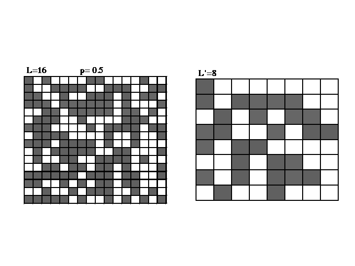
For Renormalization one must consider what size of
renormalization you are going to perform. Let us consider a b=2 type
RNG, where a you half the size of square under consideration each RNG.
As such we must consider all 2 x 2 clusters and how they
span (or occupy) in the bottom to top direction to obtain percolation.
They each have a Total occupation probability given by
the product of the individual site occupations.
The pertinent vertically spanning clusters that
renormalizes to a single shaded square (and produced
the first RNG image from L=16 to L=8) are obvious, i.e.
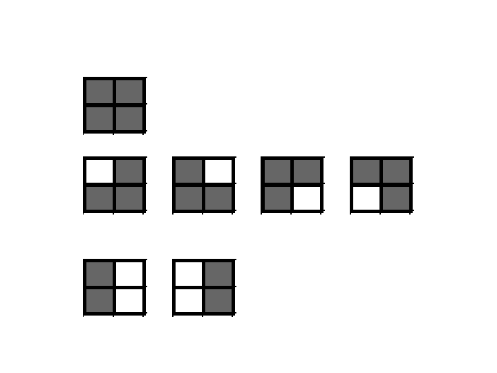
First cluster has probability of p4 ,
second set of clusters have 4 p3(1 - p) ,
last set of clusters have 2 p2(1 - p)2 ,
in order to span from bottom to top.
The new (renormalized) cell dimension is obvious reduced by
a factor of b. For example, beginning with L=16 and with
one renormalization, the new cell is L=8, which is shown in first image.
The renormalization transformation between p' and p must
reflect the connectedness, i.e. formation
of the spanning path which percolates from top to bottom, and we
define a cell to be occupied if it spans the cell vertically. This
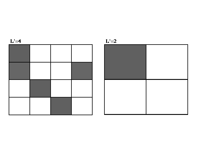
is how the L=8 square was found. Such an RNG can be performed
until we get to L=2, as the final two RNG process are shown in next
image.
The Renormalization Group Equation
Hence, if sites are occupied with probability p,
then the cells are occupied with probability p'. As a result,
the RG Equation is p' = R(p).
Hence, for the above vertically spanning clusters we have
p' = R(p) = p4 + 4 p3(1 - p) +
2 p2(1 - p)2.
The Trivial Fixed Points
Let p= p0 = 0.5, as in the images.
- One application of RG Equation gives p1 = R(0.5) = 0.44.
- Second application gives p2 = R(p1) = 0.35.
- Continued application of RG yields p = 0.
Let p= p0 = 0.7.
- Succussive RG applications gives p = 1.
These two solutions of RG Equation are called Trivial Fixed Points
because starting with anything above (or below) the p* percolation threshhold
(yet to be found) leads to these two un-interesting values. Recall
p=0 is no sites are occupied and p=1 is fully occupied.
By the way, it should be clear from the last image for p = 0.5 RNG that
there is no percolation because the last renormalization from L=2 to L=1
yields an empty site. What is p*?
The Non-Trivial Fixed Point
We want the non-trivial fixed point such that p* = R(p*).
In the present case, it is a fourth-degree polynomial, as seen from above.
Realize this depends on the size, b, of the renormalization.
Solution of this polynomial root equation yields p* = 0 and 1
(the trivial fixed points) and p* = 0.61804 . Try it!
We now associate the non-trivial fixed point, p*, with pC
the critical point. The best know value for pC = 0.5927.
So, with such a simple b=2 RG, we find a very good estimate (4% error)
of the critical point. Similar results may be found in the
thermodynamic version of RNG.
For an introduction into a thermodynamic version of RNG,
where the partition function is renormalized to obtain a
scaled interaction (so-called coupling constant) and the
RG Equation for the partition function, see
R.J. Creswick, H.A. Farach, C.P. Poole, Jr.,
Introduction to Renormalization Group Methods in Physics.
The algebra is straightforward in the nearest-neighbor Ising
case for a 1 and 2 Dimension, but grungy.
Back to the Calendar
November 8, 1999 by Duane Johnson.