 .
.
See the formula page. Readings A & T
pgs. 58-64, 185-191
This lecture continues the discussion of the calculation of properties, in particular the calculation of dynamical properties and the response to perturbation. For static properties it would probably be more convenient to do Monte Carlo methods since they are more robust. Dynamics is the reason that we do MD.
The simplest dynamical properties are the linear response to an external perturbation. Most macroscopic measurements are in the linear regime because macroscopic perturbations are very small on the scale of microscopic forces.
Onsager's made a well known conjecture (1935), called the Regression Hypothesis. (also known as the fluctuation-dissipation theorem.) It states that the linear response of the system to a time-varying perturbation is the same as fluctuations that naturally occur in statistical equilibrium. So there are 2 basic ways to calculate response: either wait for the system to fluctuate by itself or apply a perturbation and see what happens. (the first is often referred to as the Kubo method.)
First let us consider static perturbations. Suppose our total Hamiltonian has the form:
H = H0 + c A
where H0 is the unperturbed Hamiltonian, A is a perturbation and 'c' is the coupling constant. As shown on the formula page one can write the free energy as a power series in 'c'. The linear response is simply the expectation of A in the unperturbed system. The second order term is the fluctuation about the mean. In fact if we neglect all terms above the first order we always get an upper bound to the free energy. Finally to calculate the free energy difference between the system at c=0 and c=1 we just need to integrate the average A over ensembles for various values of c between 0 and 1.
We can also find the response of some property (B) to the perturbation; it equals the correlation between A and B.
In class I did the application of cutting off the potential. Generally one expects that if the neglected potential is smooth it is pretty much independent of the phase space point R, and hence terms higher order than first can be neglected.
A second example is to apply a sinusoidal potential and look at the response of the density. It is simply S k, the structure factor. That is essentially how neutrons and X-rays measure the structure factor.
Now consider the simplest dynamical experiment, mix two types of atoms and see how quickly diffusion makes the system a homogeneous mixture. The diffusion constant D, together with the diffusion equation, governs this process on a macroscopic scale. The Green's function for the diffusion equation is a spreading Gaussian with the mean squared displacement equal to 6 D t. A little thought shows that a way to microscopically calculate D is to study the diffusion of a single atom. Again the equation is on the formula page. One can easily transform this expression to the integral of the velocity autocorrelation function.
The transformation assumes that
one is using the unwound coordinates; the positions of the atoms such
that:
r(t+h) = r(t) + h v(t) + ...
Don't use periodic boundary
conditions to put particles back in the central cell.
One of the key discoveries in the early days of computer simulation was the long-time tails on the v-v function. by Alder and Wainwright. The v-v correlation functions decay algebraically in time. (as t-d/2) where d is the spatial dimension.) This implies that diffusion may not really exist in 2D. This is not Markovian (random) behavior which would decay exponentially in time. The momentum of a fast moving particle gets stored in the nearby liquid as a vortex and helps to keep it moving in the same direction for a very long time. (citation)
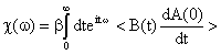
If we measure the response to A of a perturbation B it is the correlation between A and the time derivative of B (or vice versa) which enters. The coefficent (called chi) or the susceptibility is the linear response, or transport coefficient. Some examples are the electrical and thermal conductivity, the bulk and shear viscosity, the mass diffusion coefficient and the dynamical structure factor. . In linear response the perturbation and the response are at the same frequency and wavelength. Macroscopically one is often interested in only the zero-frequency, zero-wavelength limit of the response. A peak at finite frequency shows the presence of a collective mode, for example a sound wave. The derivation of the fluctuation dissipation theorem is in many textbooks (citation). The general result for a perturbation is
.
The dynamic structure factor is a key quantity (also known as the density-density response function). If you push the system at time and place (r,t) how does it respond at (r',t')? This is what neutron scattering does. It is not hard to see that sound waves of various kinds will show up as prominent features of Sk (w). The book The Theory of Simple Liquids by Hansen and MacDonald contains a thorough treatment of the theoretical properties of this function.
The Time correlation functions given by CAB(T)= < A(t)B(t + T)>. As this is an equilibrium property and it depends only on the time delay, T, this must be independent of time origin, t. This means that the function C(T) is stationary with respect to time origin, or d/dt C(T) = 0. This time-origin invariance can be seen as C(T)= <A(t) B(t + T)> = <A(t + s) B(t + s + T)>. Let s = -T, then C(T)= <A(t - T) B(t)>. In other words, you either shift B forward by time delay T, or A backwards by T, both are same average.
For T=0, C(0) = <A(t)B(t)>, and this is the time-averaged pair-correlation that we normally calculated for thermodynamic quantities, etc. Here it is important to note that for non-periodic or chaotic functions, limit of t-> infinity C(0)=<A><B>, whereas for periodic functions (which are not ergodic) this is not true. Typically, we choose to normalized the time correlation functions by C(0), i.e. c(T)= C(T)/C(0), so that c(T) ranges from 1 to its uncorrelated value <A><B>/<A(0)B(0)>. Clearly, in cases where either <A> or <B> are zero, such as for a non-flowing (or a stationary center-of-mass) system of particles where A=v=velocity and <v>=0, c(T) varies from 1 at time zero to 0 at long times. It can be negative in between.
One of the most important correlations is the auto-correlation
function, which is defined as <A(t) A(t + T)>, the time correlation of a
function with itself. By considering <(A(t + T) - A(t))2>
which is always positive definite, we may expand and find that
it equals 2<A2(t)> - 2<A(t)A(t + T)>.
Hence, the normalized auto-correlation function is bounded,
i.e. |c(T)| < or = 1.
For dynamics, one example is that velocity-velocity autocorrelation
functions Cvv(T)=<vi(T) * vi(0)>,
which is related to the Diffusion coefficient. So Cvv(T) is
1 at T=0 and <vi>2 at long times.
Importantly, for indistinguishable particles, statistical precision is
improved greatly if one considers that average over all particles in the
simulation , i.e.
(1/N)  i <(vi(T) * vi(0
)>.
i <(vi(T) * vi(0
)>.